In [ ]:
import numpy as np
import sklearn
from sklearn.model_selection import train_test_split
from sklearn.metrics import classification_report, mean_squared_error, roc_curve, auc
import seaborn as sn
import matplotlib.pyplot as plt
import pandas as pd
import shap
from keras.layers import Input, Dense, Flatten, \
    Concatenate, concatenate, Dropout, Lambda
from keras.models import Model, Sequential
from keras.layers.embeddings import Embedding
import keras
from livelossplot import PlotLossesKeras
import eli5
from eli5.sklearn import PermutationImportance
import scipy
from scipy.cluster import hierarchy as hc
from lime.lime_tabular import LimeTabularExplainer
import math
import xai
import alibi

params = {
          "ytick.color" : "w",
          "xtick.color" : "w",
          "text.color": "white",
          'figure.facecolor': "#384151",
          'legend.facecolor': "#384151",
          "axes.labelcolor" : "w",
          "axes.edgecolor" : "w",
          'font.size': '20.0',
          'figure.figsize': [20, 7],
    }

plt.rcParams.update(params)


shap.initjs()


label_column = "loan"
csv_path = 'data/adult.data'
csv_columns = ["age", "workclass", "fnlwgt", "education", "education-num", "marital-status",
                   "occupation", "relationship", "ethnicity", "gender", "capital-gain", "capital-loss",
                   "hours-per-week", "native-country", "loan"]
input_columns = ["age", "workclass", "education", "education-num", "marital-status",
                   "occupation", "relationship", "ethnicity", "gender", "capital-gain", "capital-loss",
                   "hours-per-week", "native-country"]
categorical_features = ["workclass", "education", "marital-status",
                       "occupation", "relationship", "ethnicity", "gender",
                       "native-country"]

def prepare_data(df):

    if "fnlwgt" in df: del df["fnlwgt"]

    tmp_df = df.copy()

    # normalize data (this is important for model convergence)
    dtypes = list(zip(tmp_df.dtypes.index, map(str, tmp_df.dtypes)))
    for k,dtype in dtypes:
        if dtype == "int64":
            tmp_df[k] = tmp_df[k].astype(np.float32)
            tmp_df[k] -= tmp_df[k].mean()
            tmp_df[k] /= tmp_df[k].std()

    cat_columns = tmp_df.select_dtypes(['object']).columns
    tmp_df[cat_columns] = tmp_df[cat_columns].astype('category')
    tmp_df[cat_columns] = tmp_df[cat_columns].apply(lambda x: x.cat.codes)
    tmp_df[cat_columns] = tmp_df[cat_columns].astype('int8')

    return tmp_df

def get_dataset_1():
    tmp_df = df.copy()
    tmp_df = tmp_df.groupby('loan') \
                .apply(lambda x: x.sample(100) if x["loan"].iloc[0] else x.sample(7_900)) \
                .reset_index(drop=True)

    X = tmp_df.drop(label_column, axis=1).copy()
    y = tmp_df[label_column].astype(int).values.copy()

    return tmp_df, df_display.copy()

def get_production_dataset():
    tmp_df = df.copy()
    tmp_df = tmp_df.groupby('loan') \
                .apply(lambda x: x.sample(50) if x["loan"].iloc[0] else x.sample(60)) \
                .reset_index(drop=True)

    X = tmp_df.drop(label_column, axis=1).copy()
    y = tmp_df[label_column].astype(int).values.copy()

    return X, y


def get_dataset_2():
    tmp_df = df.copy()
    tmp_df_display = df_display.copy()
#     tmp_df_display[label_column] = tmp_df_display[label_column].astype(int).values

    X = tmp_df.drop(label_column, axis=1).copy()
    y = tmp_df[label_column].astype(int).values.copy()

    X_display = tmp_df_display.drop(label_column, axis=1).copy()
    y_display = tmp_df_display[label_column].astype(int).values.copy()

    X_train, X_valid, y_train, y_valid = \
        train_test_split(X, y, test_size=0.2, random_state=7)

    return X, y, X_train, X_valid, y_train, y_valid, X_display, y_display, tmp_df, tmp_df_display

df_display = pd.read_csv(csv_path, names=csv_columns)
df_display[label_column] = df_display[label_column].apply(lambda x: ">50K" in x)
df = prepare_data(df_display)

def build_model(X):
    input_els = []
    encoded_els = []
    dtypes = list(zip(X.dtypes.index, map(str, X.dtypes)))
    for k,dtype in dtypes:
        input_els.append(Input(shape=(1,)))
        if dtype == "int8":
            e = Flatten()(Embedding(df[k].max()+1, 1)(input_els[-1]))
        else:
            e = input_els[-1]
        encoded_els.append(e)
    encoded_els = concatenate(encoded_els)

    layer1 = Dropout(0.5)(Dense(100, activation="relu")(encoded_els))
    out = Dense(1, activation='sigmoid')(layer1)

    # train model
    model = Model(inputs=input_els, outputs=[out])
    model.compile(optimizer="adam", loss='binary_crossentropy', metrics=['accuracy'])
    return model

def f_in(X, m=None):
    """Preprocess input so it can be provided to a function"""
    if m:
        return [X.iloc[:m,i] for i in range(X.shape[1])]
    else:
        return [X.iloc[:,i] for i in range(X.shape[1])]

def f_out(probs):
    """Convert probabilities into classes"""
    return list((probs >= 0.5).astype(int).T[0])

def plot_roc(y, probs):

    fpr, tpr, _ = roc_curve(y, probs)

    roc_auc = auc(fpr, tpr)
    print(roc_auc)

    plt.figure()
    plt.plot(fpr, tpr, label='ROC curve (area = %0.2f)' % roc_auc)
    plt.plot([0, 1], [0, 1], 'k--')
    plt.xlim([0.0, 1.0])
    plt.ylim([0.0, 1.05])
    plt.xlabel('False Positive Rate')
    plt.ylabel('True Positive Rate')
    plt.title('ROC curve (area = %0.2f)' % roc_auc)
    plt.legend(loc="lower right")
    plt.rcParams.update(params)
    plt.show()

def plot_learning_curves(model, X, y):
    X_train, X_val, y_train, y_val = train_test_split(X, y, test_size=0.2)
    train_errors, val_errors = [], []
    for m in list(np.logspace(0.6,4,dtype='int')):
        if m >= len(X_train): break
        model.fit(f_in(X_train,m), y_train[:m], epochs=50, batch_size=512, verbose=0)
        y_train_predict = model.predict(f_in(X_train,m))
        y_val_predict = model.predict(f_in(X_val))
        y_train_predict = f_out(y_train_predict)
        y_val_predict = f_out(y_val_predict)
        train_errors.append(mean_squared_error(y_train[:m], y_train_predict))
        val_errors.append(mean_squared_error(y_val, y_val_predict))
    plt.plot(np.sqrt(train_errors), "r-+", linewidth=2, label="train")
    plt.plot(np.sqrt(val_errors), "b-", linewidth=3, label="val")

def keras_score(self, X, y, **kwargs):
    """ Scorer class for eli5 library on feature importance"""
    input_test = [X[:,i] for i in range(X.shape[1])]
    loss = self.evaluate(input_test, y)
    if type(loss) is list:
        # The first one is the error, the rest are metrics
        return -loss[0]
    return -loss

class ModelWrapper():
    """ Keras model wrapper to override the predict function"""
    def __init__(self, model):
        self.model = model

    def predict(self, X, **kwargs):
        return self.model.predict([X.iloc[:,i] for i in range(X.shape[1])])

def plot_all_features(X, plot_numeric=True, hist=True, dropna=False):
    fig = plt.figure(figsize=(20,15))
    cols = 5
    rows = math.ceil(float(X.shape[1]) / cols)
    for i, column in enumerate(X.columns):
        ax = fig.add_subplot(rows, cols, i + 1)
        ax.set_title(column)
        if X.dtypes[column] == np.object:
            X[column].value_counts().plot(kind="bar", axes=ax)
        elif plot_numeric:
            if hist:
                X[column].hist(axes=ax)
                plt.xticks(rotation="vertical")
            else:
                if dropna:
                    X[column].dropna().plot()
                else:
                    X[column].plot()

    plt.subplots_adjust(hspace=0.7, wspace=0.2)

def plot_dendogram(corr, X):
    corr_condensed = hc.distance.squareform(1-corr)
    z = hc.linkage(corr_condensed, method="average")
    fig = plt.figure(figsize=(16,5))
    dendrogram = hc.dendrogram(
        z, labels=X.columns, orientation="left", leaf_font_size=16)
    plt.show()

def shap_predict(X):
    values = model.predict([X[:,i] for i in range(X.shape[1])]).flatten()
    return values

def lime_predict_proba(X):
    values = model.predict([X[:,i] for i in range(X.shape[1])]).flatten()
    prob_pairs = np.array([1-values, values]).T
    return prob_pairs


import alibi
import numpy as np
from sklearn.preprocessing import LabelEncoder, StandardScaler, OneHotEncoder
from sklearn.impute import SimpleImputer
from sklearn.pipeline import Pipeline
from sklearn.compose import ColumnTransformer
from sklearn.ensemble import RandomForestClassifier

alibi_data, alibi_labels, alibi_feature_names, alibi_category_map = alibi.datasets.adult()

def get_alibi_data():

    # define train and test set
    np.random.seed(0)
    data_perm = np.random.permutation(np.c_[alibi_data, alibi_labels])
    data = data_perm[:, :-1]
    labels = data_perm[:, -1]

    idx = 30000
    X_train, y_train = data[:idx, :], labels[:idx]
    X_test, y_test = data[idx + 1:, :], labels[idx + 1:]

    # feature transformation pipeline
    ordinal_features = [x for x in range(len(alibi_feature_names)) if x not in list(alibi_category_map.keys())]
    ordinal_transformer = Pipeline(steps=[('imputer', SimpleImputer(strategy='median')),
                                          ('scaler', StandardScaler())])

    categorical_features = list(alibi_category_map.keys())
    categorical_transformer = Pipeline(steps=[('imputer', SimpleImputer(strategy='median')),
                                              ('onehot', OneHotEncoder(handle_unknown='ignore'))])

    preprocessor = ColumnTransformer(transformers=[('num', ordinal_transformer, ordinal_features),
                                                   ('cat', categorical_transformer, categorical_features)])


    np.random.seed(0)
    clf = RandomForestClassifier(n_estimators=50)

    alibi_loan_model = Pipeline(steps=[
        ('preprocessor', preprocessor),
        ('clf', clf)])

    alibi_loan_model.fit(X_train, y_train)

    return X_train, X_test, y_train, y_test, \
        alibi_category_map, alibi_feature_names, alibi_loan_model

X_train_alibi, X_test_alibi, y_train_alibi, y_test_alibi, \
    category_map_alibi, feature_names_alibi, loan_model_alibi = get_alibi_data()


import tensorflow as tf
tf.logging.set_verbosity(tf.logging.ERROR)  # suppress deprecation messages
from tensorflow.keras.models import load_model
from tensorflow.keras.utils import to_categorical

from alibi.explainers import CounterFactual

# def cnn_model():
#     from tensorflow.keras import backend as K
#     from tensorflow.keras.layers import Conv2D, Dense, Dropout, Flatten, MaxPooling2D, Input, UpSampling2D
#     from tensorflow.keras.models import Model
#     x_in = Input(shape=(28, 28, 1))
#     x = Conv2D(filters=64, kernel_size=2, padding='same', activation='relu')(x_in)
#     x = MaxPooling2D(pool_size=2)(x)
#     x = Dropout(0.3)(x)
#     x = Conv2D(filters=32, kernel_size=2, padding='same', activation='relu')(x)
#     x = MaxPooling2D(pool_size=2)(x)
#     x = Dropout(0.3)(x)
#     x = Flatten()(x)
#     x = Dense(256, activation='relu')(x)
#     x = Dropout(0.5)(x)
#     x_out = Dense(10, activation='softmax')(x)
#     cnn = Model(inputs=x_in, outputs=x_out)
#     cnn.compile(loss='categorical_crossentropy', optimizer='adam', metrics=['accuracy'])
#     return cnn

# cnn = cnn_model()
# cnn.summary()
# cnn.fit(x_train, y_train, batch_size=64, epochs=3, verbose=0)
# cnn.save('mnist_cnn.h5')

def show_iterations(explanation, max_lam_steps=10):
    n_cfs = np.array([len(explanation['all'][iter_cf]) for iter_cf in range(max_lam_steps)])
    examples = {}
    for ix, n in enumerate(n_cfs):
        if n>0:
            examples[ix] = {'ix': ix, 'lambda': explanation['all'][ix][0]['lambda'],
                           'X': explanation['all'][ix][0]['X']}
    columns = len(examples) + 1
    rows = 1

    fig = plt.figure(figsize=(16,6))

    for i, key in enumerate(examples.keys()):
        ax = plt.subplot(rows, columns, i+1)
        ax.get_xaxis().set_visible(False)
        ax.get_yaxis().set_visible(False)
        plt.imshow(examples[key]['X'].reshape(28,28))
        plt.title(f'Iter {key}')

(cf_x_train, cf_y_train), (cf_x_test, cf_y_test) = tf.keras.datasets.mnist.load_data()
print('x_train shape:', cf_x_train.shape, 'y_train shape:', cf_y_train.shape)
plt.gray()

cf_x_train = cf_x_train.astype('float32') / 255
cf_x_test = cf_x_test.astype('float32') / 255
cf_x_train = np.reshape(cf_x_train, cf_x_train.shape + (1,))
cf_x_test = np.reshape(cf_x_test, cf_x_test.shape + (1,))
cf_y_train = to_categorical(cf_y_train)
cf_y_test = to_categorical(cf_y_test)

cf_xmin, cf_xmax = -.5, .5
cf_x_train = ((cf_x_train - cf_x_train.min()) / (cf_x_train.max() - cf_x_train.min())) * (cf_xmax - cf_xmin) + cf_xmin
cf_x_test = ((cf_x_test - cf_x_test.min()) / (cf_x_test.max() - cf_x_test.min())) * (cf_xmax - cf_xmin) + cf_xmin
Hype-ML - A NEW Project has come in!
- Insurance company has a process where domain expert approves/rejects loan applications
- They receive over 1m applications and want to automate the process
Business wants it NOW!
- They heard their competitor is using "Machine Learning" and business says we need to use that

In [160]:
df_data, df_display = get_dataset_1()

df_display.head()
Out[160]:
In [161]:
X = df_data.drop(label_column, axis=1).copy()
y = df_data[label_column].astype(int).values.copy()
X_train, X_valid, y_train, y_valid = \
train_test_split(X, y, test_size=0.2, random_state=7)
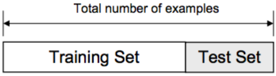
print("Training size:", y_train.shape, "Testing size: ", y_valid.shape)
In [162]:
# 1 layer, 100 neurons model, with softmax (0-1 probabilities)
model = build_model(X)

model.fit(f_in(X_train), y_train, epochs=10,
    batch_size=512, shuffle=True, validation_data=(f_in(X_valid), y_valid),
    callbacks=[PlotLossesKeras()], verbose=0, validation_split=0.05,)

Out[162]:
In [163]:
score = model.evaluate(f_in(X_valid), y_valid, verbose=1)
print("Error %.4f: " % score[0])
print("Accuracy %.4f: " % (score[1]*100))
In [164]:
X_prod, y_prod = get_production_dataset()

print(X_prod.shape)
X_prod.head()
Out[164]:
In [165]:
probabilities = model.predict(f_in(X_prod))
pred = f_out(probabilities)
_= xai.metrics_plot(pred, y_prod, exclude_metrics=["auc", "specificity", "f1"])

In [166]:
xai.confusion_matrix_plot(y_prod, pred)

In [167]:
fig, ax = plt.subplots(1,2)
a = sn.countplot(y_valid, ax=ax[0]); a.set_title("TRAINING DATA"); a.set_xticklabels(["Rejected", "Approved"])
a = sn.countplot(y_prod, ax=ax[1]); a.set_title("PRODUCTION"); a.set_xticklabels(["Rejected", "Approved"])
Out[167]:


Undesired bias and explainability
Has become popular due to several high profile incidents:
- Amazon's "sexist" recruitment tool
- Microsoft's "racist" chatbot
- Negative discrimination in automated sentencing
- Black box models + complex patterns can't be interpretable
Organisations cannot take on unknown risks


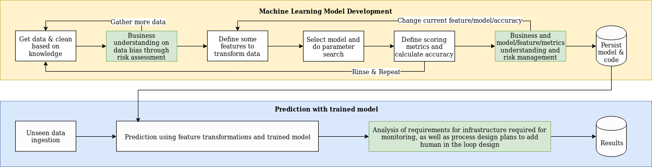
Stages where bias can appear
1) Statistical bias (During the project)
Sub-optimal choices on decisions after project starts (models, metrics, human-in-the-loop, infrastructure design, etc)
2) A-priori bias (Before the project)
Limitations around the project that constrain the best possible outcome (limited time, budget, data, societal shifts in perception, etc)
Not as easy as just "removing bias"
- Any non trivial decision holds a bias, without exceptions - unless you build a classifier that only predicts "maybe".
- It's impossible to "just remove bias" (as the whole purpose of ML is to discriminate towards the right answer)
- Societal bias carries an inherent bias - what may be "racist" for one person, may not be for another group or geography
Emphasis on last point: Societal bias is inherently biased
What it's about: Mitigating undesired bias through process and explainability techniques
- Like in cybersecurity, it's impossible to build a system that will never be hacked
- But it's possible to build a system and introduce processes that ensure a reasonable level of security
- Similarly we want to introduce processes that allow us to remove a reasonable level of undesired biases
- This is going 0 to 1, trying to introduce a foundation for undesired bias

The explainability tradeoff
By making introducing processes that allow us to mitigate undesired bias and increase explainability, we face severall tradeoffs:
- More redtape introduced
- Potentially lower accuracy
- Constrains on models that can be used
- Increase in infrastructure complexity
- Requirement of domain expert knowledge intersection
The amount of explainability and process is proportionate to the impact of the project (prototype vs prod)
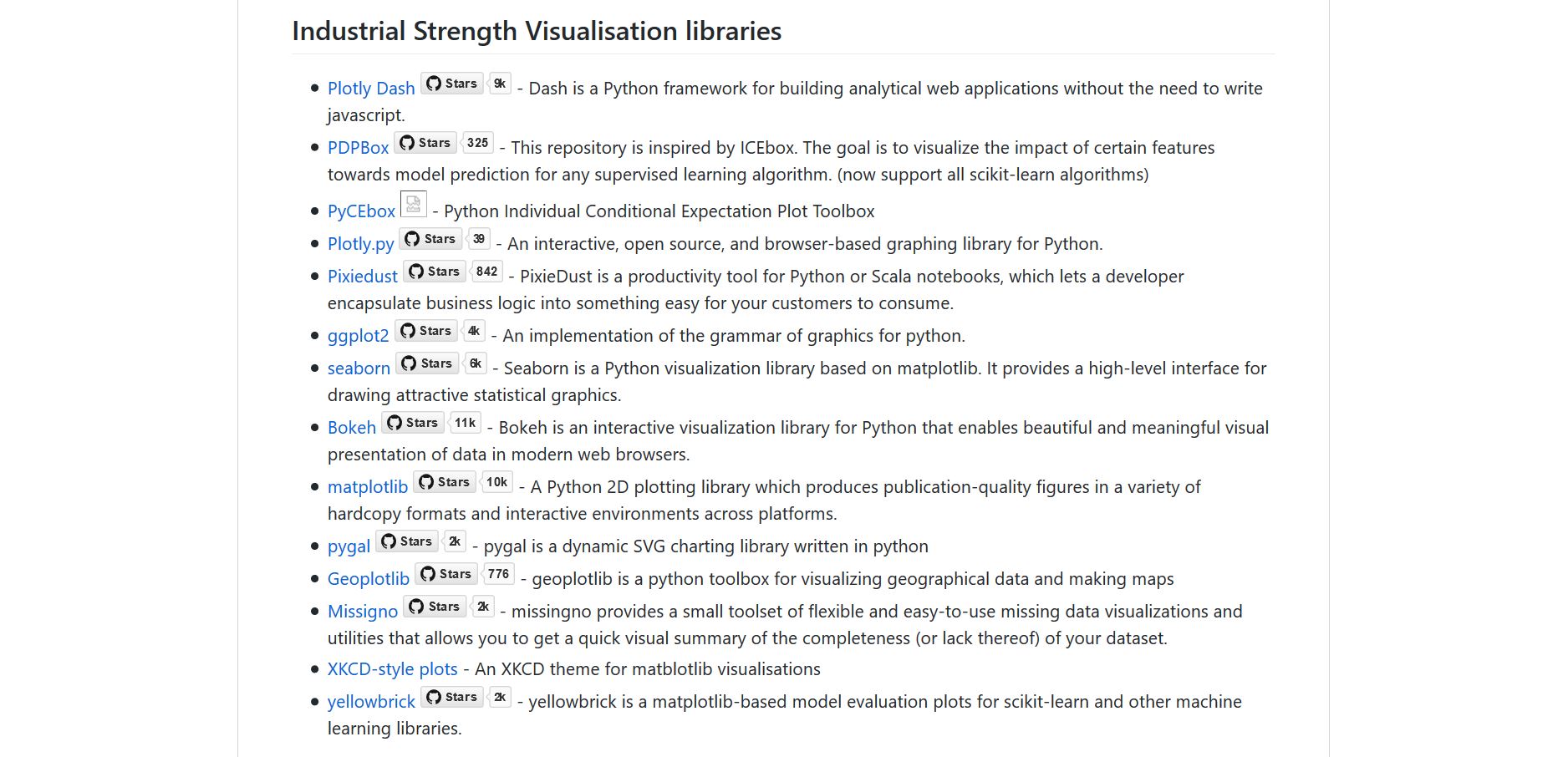
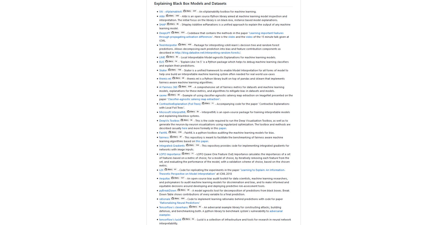
XAI - eXplainable AI
A set of tools to explain machine learning data
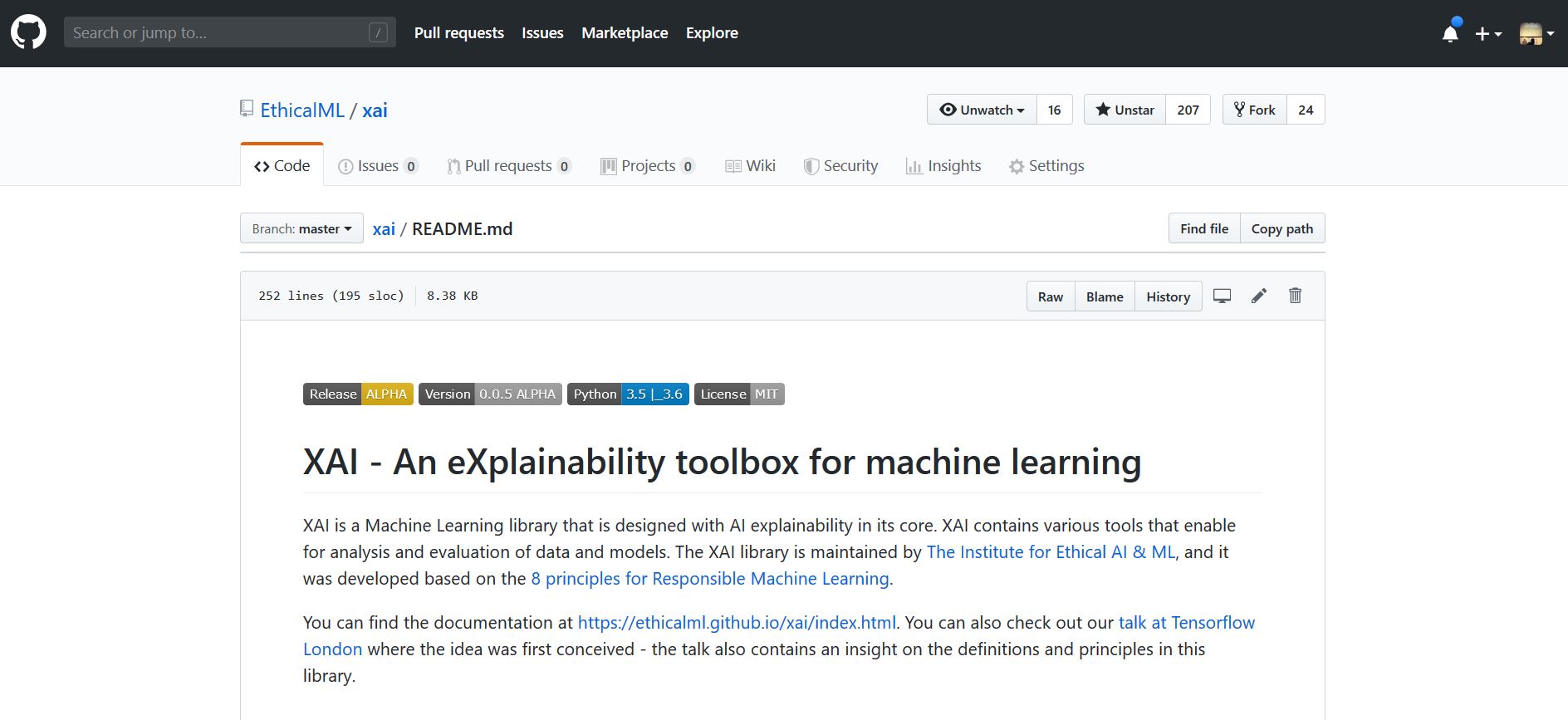
https://github.com/EthicalML/XAI
Let's get the new training dataset
In [168]:
X, y, X_train, X_valid, y_train, y_valid, X_display, y_display, df, df_display \
    = get_dataset_2()
df_display.head()
Out[168]:
In [169]:
im = xai.imbalance_plot(df_display, "gender", "loan" , categorical_cols=["loan", "gender"])

In [170]:
im = xai.balance(df_display, "gender", "loan", categorical_cols=["gender", "loan"],
                upsample=0.5, downsample=0.8)

1.2) Balanced testing / validation datasets
In [171]:
X_train_balanced, y_train_balanced, X_valid_balanced, y_valid_balanced, train_idx, test_idx = \
    xai.balanced_train_test_split(
            X, y, "gender",
            min_per_group=300,
            max_per_group=300,
            categorical_cols=["gender", "loan"])

X_valid_balanced["loan"] = y_valid_balanced
im = xai.imbalance_plot(X_valid_balanced, "gender", "loan", categorical_cols=["gender", "loan"])

In [172]:
corr = xai.correlations(df_display, include_categorical=True)

1.5 Shoutout to other tools and techniques
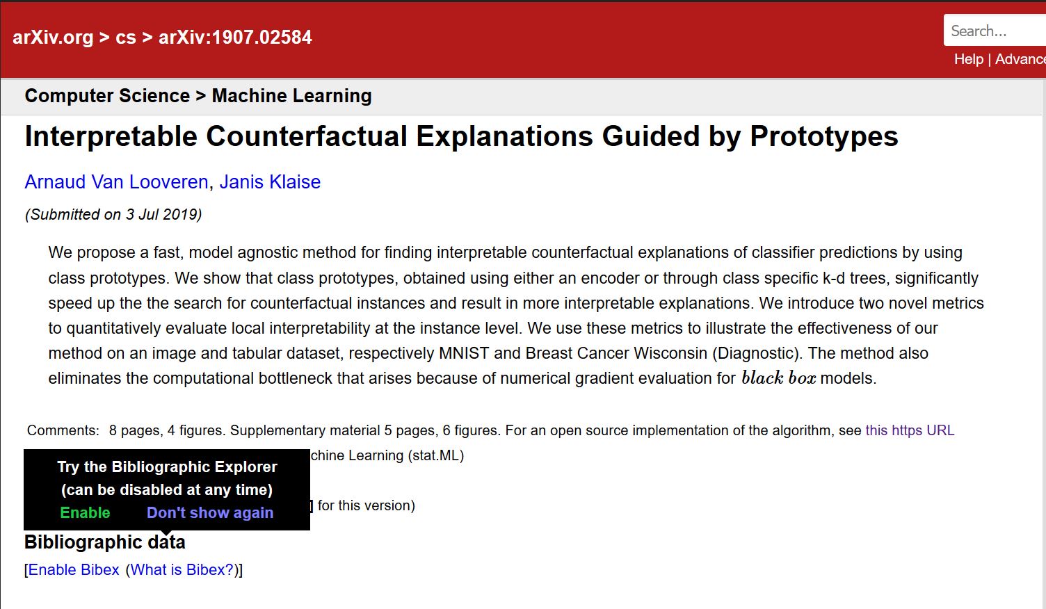
Alibi - Black Box Model Explanations
A set of proven scientific techniques to explain ML models as black boxes
https://github.com/SeldonIO/Alibi
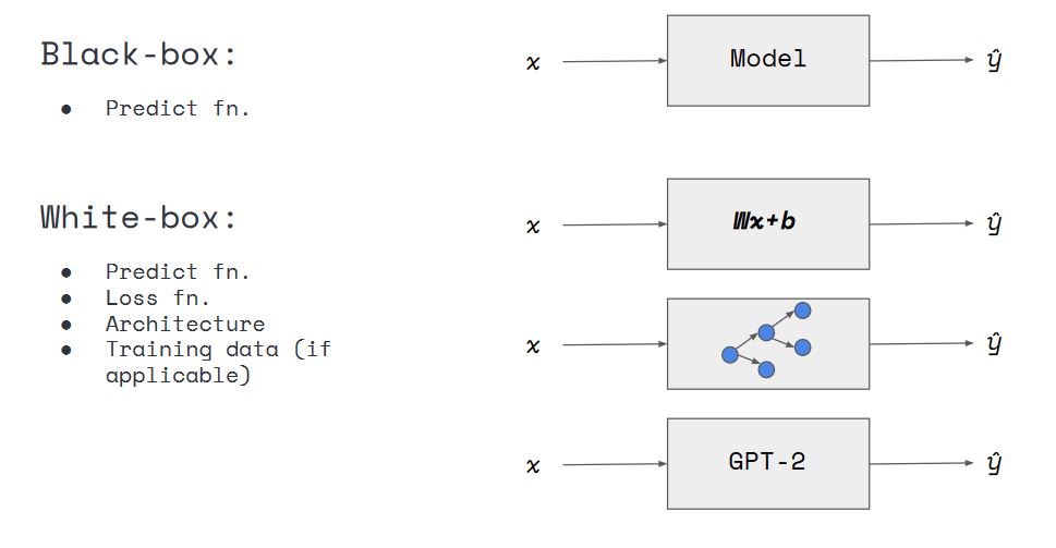
Model Evaluation Metrics: White / Black Box
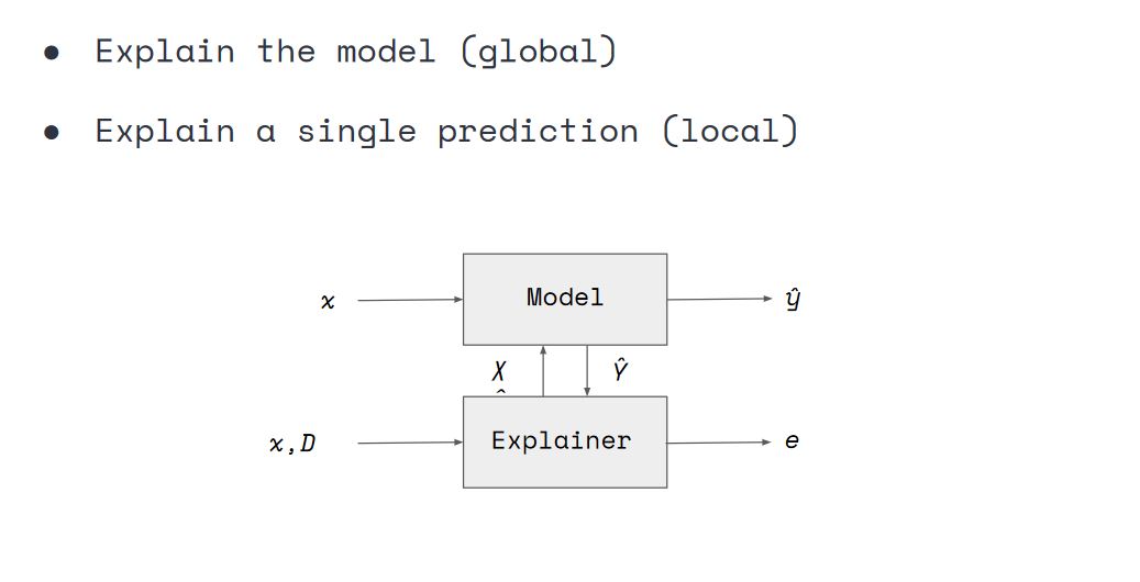
Model Evaluation Metrics: Global vs Local
Let's first train our model with the new, more reasonable dataset
In [173]:
# Let's start by building our model with our newly balanced dataset
model = build_model(X)
model.fit(f_in(X_train), y_train, epochs=20, batch_size=512, shuffle=True, validation_data=(f_in(X_valid), y_valid), callbacks=[PlotLossesKeras()], verbose=0, validation_split=0.05,)
probabilities = model.predict(f_in(X_valid))
pred = f_out(probabilities)

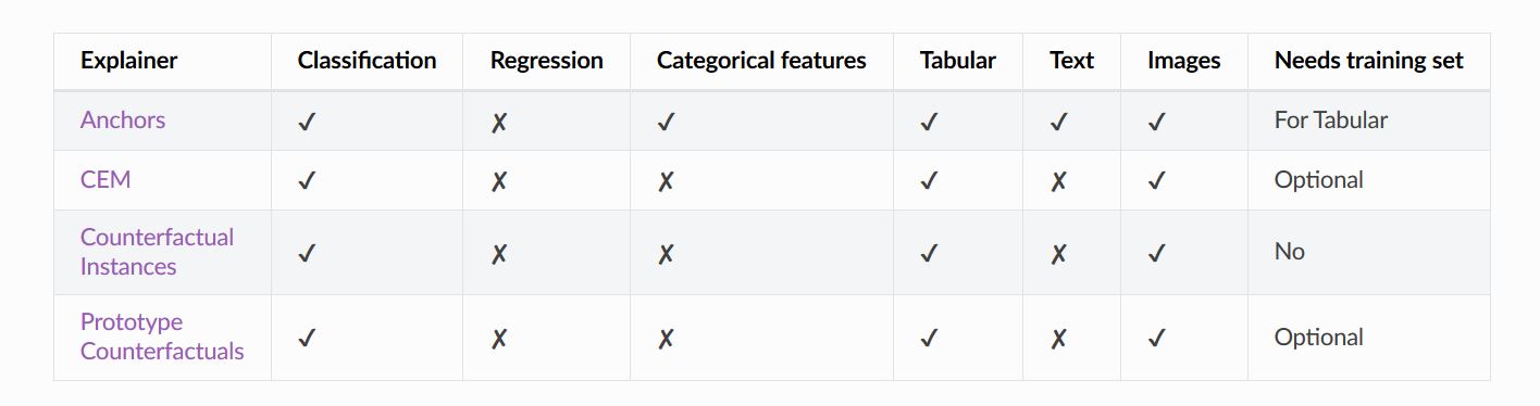
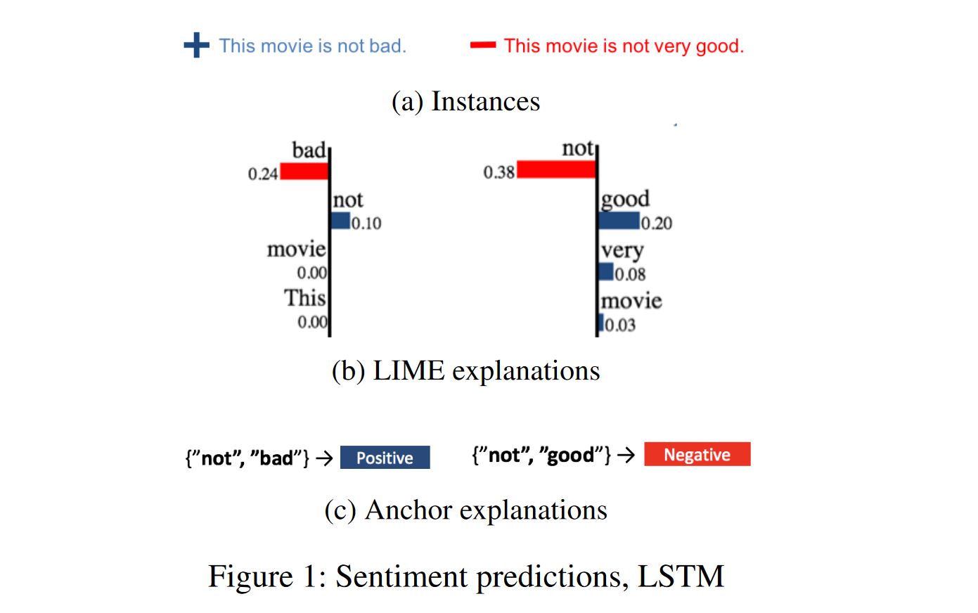
We can now use the Tabular Anchor technique in Alibi
In [174]:
from alibi.explainers import AnchorTabular

explainer = AnchorTabular(
    loan_model_alibi.predict,
    feature_names_alibi,
    categorical_names=category_map_alibi)

explainer.fit(
    X_train_alibi,
    disc_perc=[25, 50, 75])

print("Explainer built")
In [175]:
X_test_alibi[:1]
Out[175]:
In [176]:
explanation = explainer.explain(X_test_alibi[:1], threshold=0.95)

print('Anchor: %s' % (' AND '.join(explanation['names'])))
print('Precision: %.2f' % explanation['precision'])
print('Coverage: %.2f' % explanation['coverage'])
In [177]:
cnn = load_model('mnist_cnn.h5')
cf_X = cf_x_test[0].reshape((1,) + cf_x_test[0].shape)
plt.imshow(cf_X.reshape(28, 28));

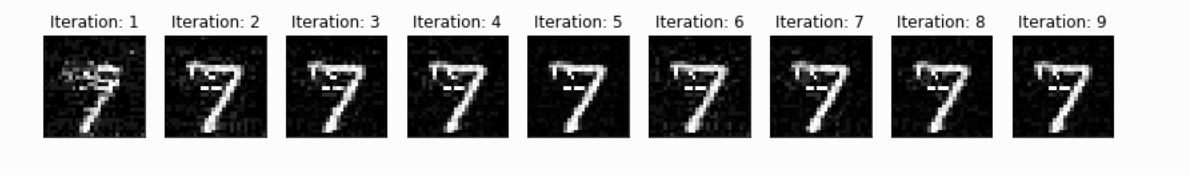
In [178]:
shape = (1,) + cf_x_train.shape[1:]
target_class = 9 # any class other than 7 will do

cf = CounterFactual(cnn, shape=shape, target_class=target_class, target_proba=1.0, max_iter=20)
explanation = cf.explain(cf_X)

print(f"Counterfactual prediction: {explanation['cf']['class']} with probability {explanation['cf']['proba'][0]}")
plt.imshow(explanation['cf']['X'].reshape(28, 28));

In [179]:
show_iterations(explanation)

Intersection with Adversarial Robustness
- Black box explainability techniques allow us to understand black boxes
- But also provide tools that could be used maliciously
- Extra considerations need to be taken into account (i.e. when is a model "being explained")
- Limited access to explainability (auditors, domain experts, etc)
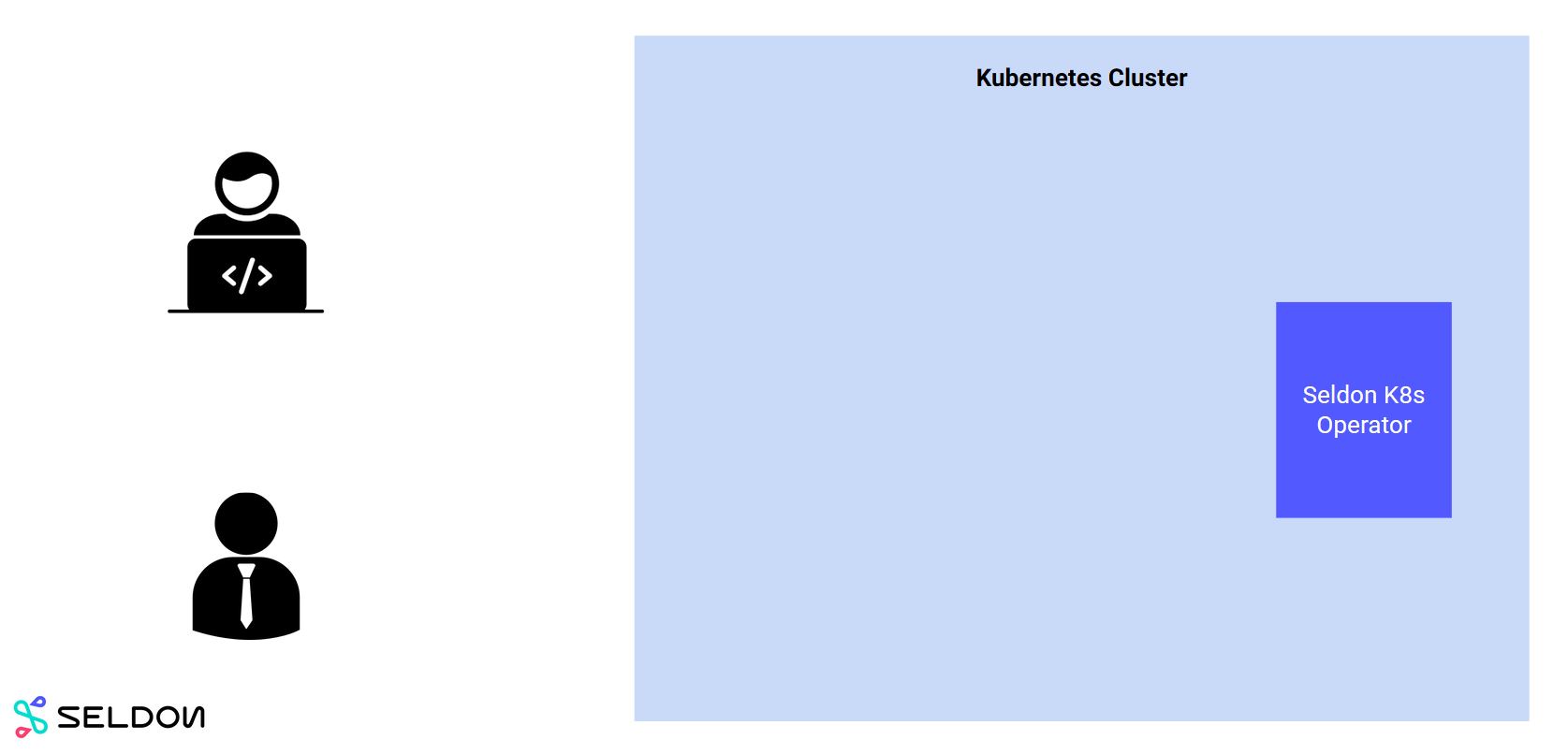
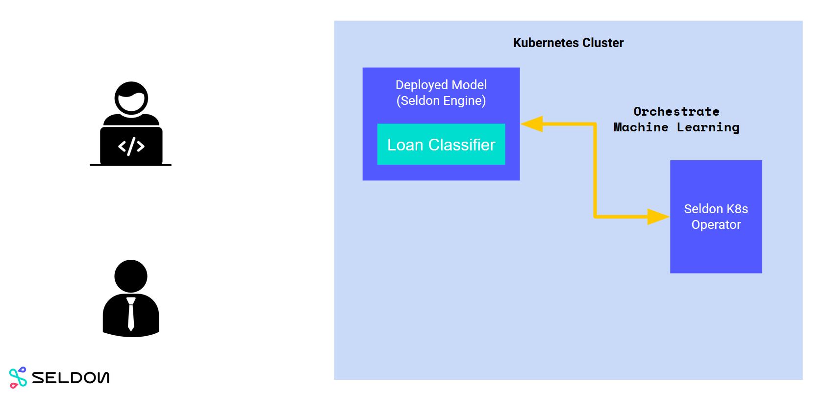
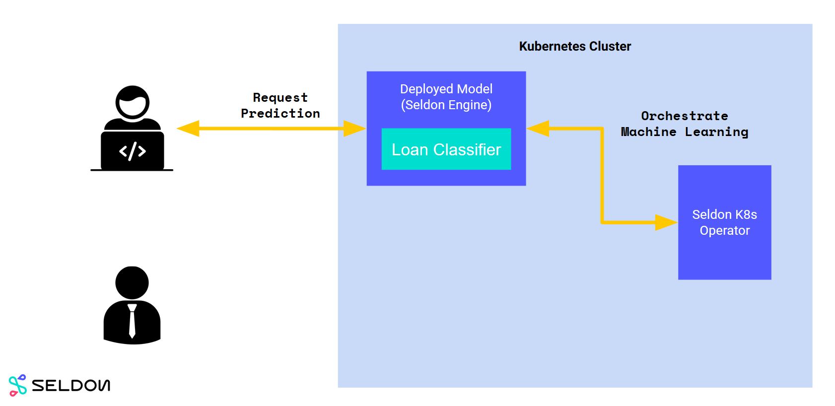
1.5 Shoutout to other tools and techniques
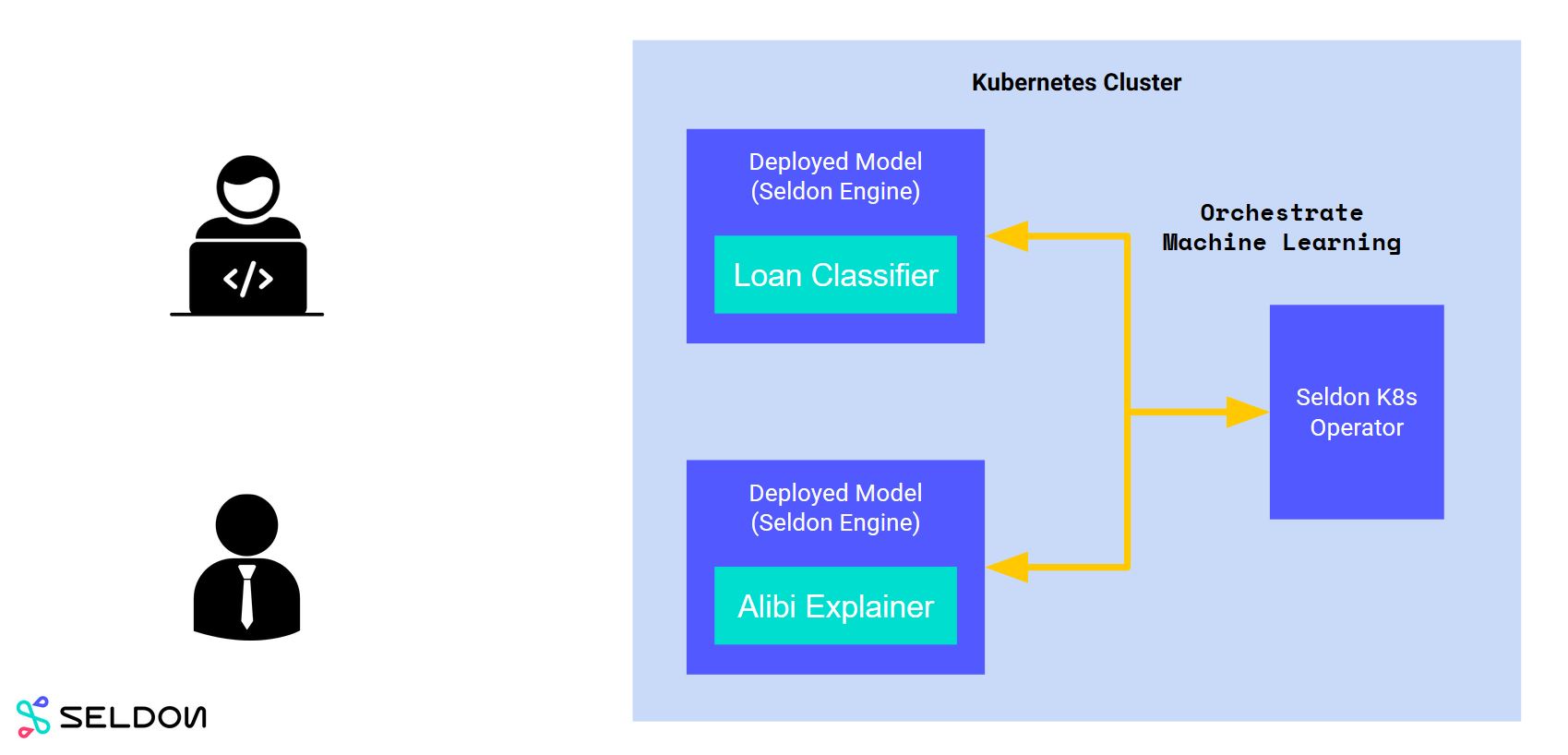
Seldon Core - Production ML in K8s
A language agnostic ML serving & monitoring framework in Kubernetes

https://github.com/SeldonIO/seldon-core
In [180]:
print(f"Input: {X_test_alibi[:1]}")
print(f"Predicted class: {randomforest.predict(preprocessor.transform(X_test_alibi[:1]))}")
print(f"Probabilities: {randomforest.predict_proba(preprocessor.transform(X_test_alibi[:1]))}")
Save the model artefacts so we can deploy them
In [ ]:
import dill

with open("pipeline/pipeline_steps/loanclassifier/preprocessor.dill", "wb") as prep_f:
    dill.dump(preprocessor, prep_f)

with open("pipeline/pipeline_steps/loanclassifier/model.dill", "wb") as model_f:
    dill.dump(randomforest, model_f)
Build a Model wrapper that uses the trained models through a predict function
In [ ]:
%%writefile pipeline/pipeline_steps/loanclassifier/Model.py
import dill

class Model:
    def __init__(self, *args, **kwargs):

        with open("preprocessor.dill", "rb") as prep_f:
            self.preprocessor = dill.load(prep_f)
        with open("model.dill", "rb") as model_f:
            self.clf = dill.load(model_f)

    def predict(self, X, feature_names=[]):
        X_prep = self.preprocessor.transform(X)
        proba = self.clf.predict_proba(X_prep)
        return proba
Add the dependencies for the wrapper to work
In [181]:
%%writefile pipeline/pipeline_steps/loanclassifier/requirements.txt
dill==0.2.9
scikit-image==0.15.0
scikit-learn==0.20.1
scipy==1.1.0
numpy==1.17.1
Use the source2image command to containerize code
In [ ]:
!s2i build pipeline/pipeline_steps/loanclassifier seldonio/seldon-core-s2i-python3:0.11 loanclassifier:0.1
Define the graph of your pipeline with individual models
In [ ]:
%%writefile pipeline/pipeline_steps/loanclassifier/loanclassifiermodel.yaml
apiVersion: machinelearning.seldon.io/v1alpha2
kind: SeldonDeployment
metadata:
  labels:
    app: seldon
  name: loanclassifier
spec:
  name: loanclassifier
  predictors:
  - componentSpecs:
    - spec:
        containers:
        - image: loanclassifier:0.1
          name: model
    graph:
      children: []
      name: model
      type: MODEL
      endpoint:
        type: REST
    name: loanclassifier
    replicas: 1
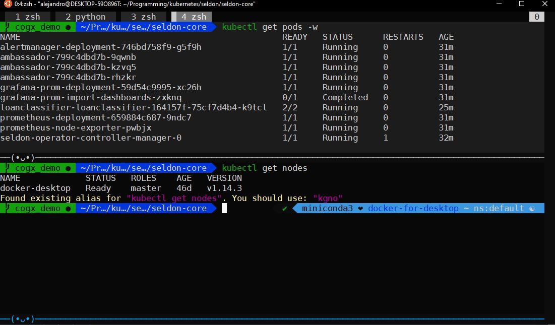
Deploy your model!
In [182]:
!kubectl apply -f pipeline/pipeline_steps/loanclassifier/loanclassifiermodel.yaml
We can now send a request through HTTP
In [183]:
batch = X_test_alibi[:1]
print(batch)
In [184]:
from seldon_core.seldon_client import SeldonClient

sc = SeldonClient(
    gateway="ambassador",
    gateway_endpoint="localhost:80",
    deployment_name="loanclassifier",
    payload_type="ndarray",
    namespace="default",
    transport="rest")

client_prediction = sc.predict(data=batch)

print(client_prediction.response.data.ndarray)
Now we can send data through the REST API
In [185]:
%%bash
curl -X POST -H 'Content-Type: application/json' \
    -d "{'data': {'names': ['text'], 'ndarray': [[52,  4,  0,  2,  8,  4,  2,  0,  0,  0, 60,  9]]}}" \
    "http://localhost:80/seldon/default/loanclassifier/api/v0.1/predictions"
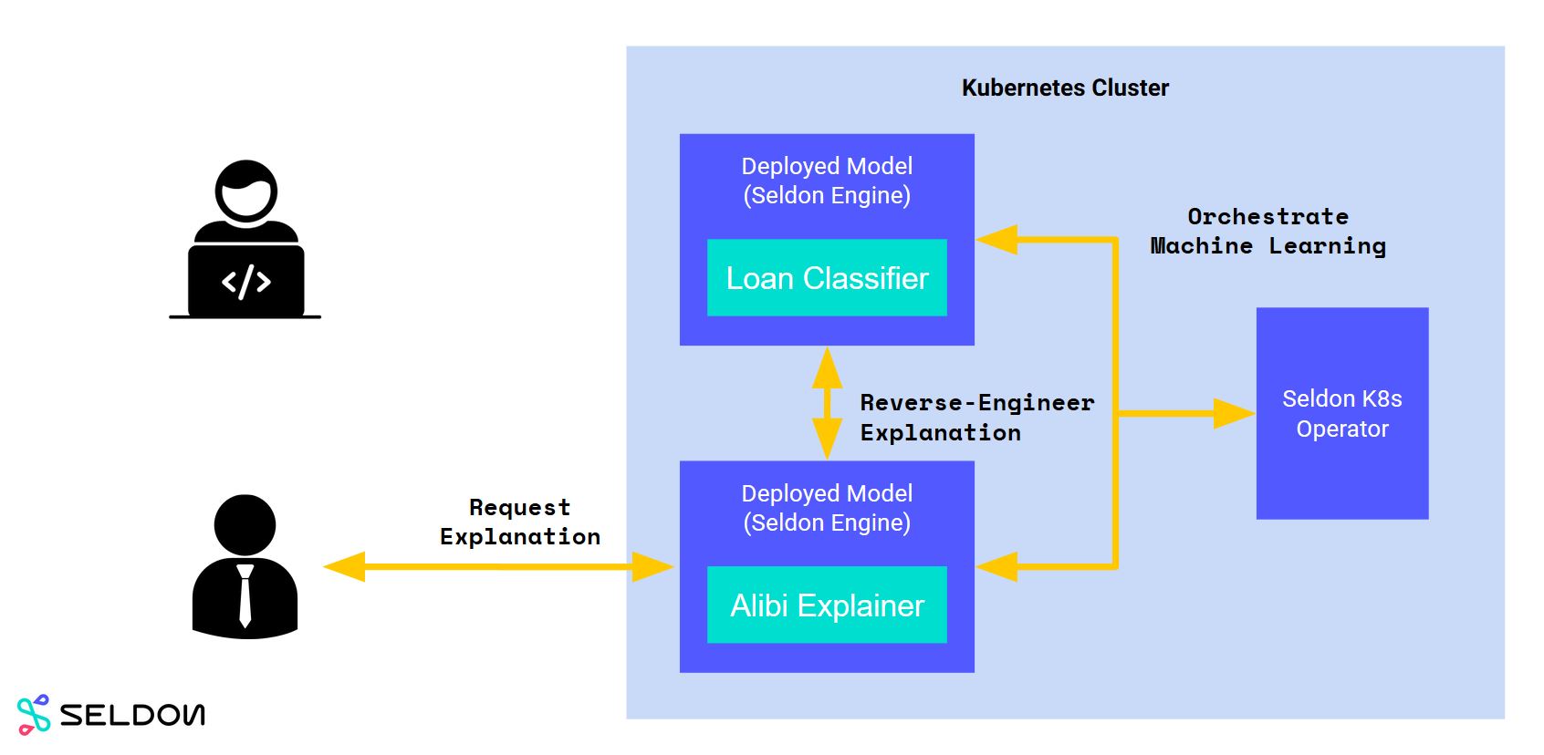
Now we can create an explainer for our model
In [186]:
from alibi.explainers import AnchorTabular

predict_fn = lambda x: randomforest.predict(preprocessor.transform(x))
explainer = AnchorTabular(predict_fn, alibi_feature_names, categorical_names=alibi_category_map)
explainer.fit(X_train_alibi, disc_perc=[25, 50, 75])

explanation = explainer.explain(X_test_alibi[0], threshold=0.95)

print('Anchor: %s' % (' AND '.join(explanation['names'])))
print('Precision: %.2f' % explanation['precision'])
print('Coverage: %.2f' % explanation['coverage'])
But now we can use the remote model we have in production
In [ ]:
def predict_remote_fn(X):
    from seldon_core.seldon_client import SeldonClient
    from seldon_core.utils import get_data_from_proto

    kwargs = {
        "gateway": "ambassador",
        "deployment_name": "loanclassifier",
        "payload_type": "ndarray",
        "namespace": "default",
        "transport": "rest"
    }

    try:
        kwargs["gateway_endpoint"] = "localhost:80"
        sc = SeldonClient(**kwargs)
        prediction = sc.predict(data=X)
    except:
        # If we are inside the container, we need to reach the ambassador service directly
        kwargs["gateway_endpoint"] = "ambassador:80"
        sc = SeldonClient(**kwargs)
        prediction = sc.predict(data=X)

    y = get_data_from_proto(prediction.response)
    return y
And train our explainer to use the remote function
In [187]:
from seldon_core.utils import get_data_from_proto

explainer = AnchorTabular(predict_remote_fn, alibi_feature_names, categorical_names=alibi_category_map)
explainer.fit(X_train_alibi, disc_perc=[25, 50, 75])

explanation = explainer.explain(batch, threshold=0.95)

print('Anchor: %s' % (' AND '.join(explanation['names'])))
print('Precision: %.2f' % explanation['precision'])
print('Coverage: %.2f' % explanation['coverage'])
To containerise our explainer, save the trained binary
In [ ]:
import dill

with open("pipeline/pipeline_steps/loanclassifier-explainer/explainer.dill", "wb") as x_f:
    dill.dump(explainer, x_f)
Expose it through a wrapper
In [ ]:
%%writefile pipeline/pipeline_steps/loanclassifier-explainer/Explainer.py
import dill
import json
import numpy as np

class Explainer:
    def __init__(self, *args, **kwargs):

        with open("explainer.dill", "rb") as x_f:
            self.explainer = dill.load(x_f)

    def predict(self, X, feature_names=[]):
        print("Received: " + str(X))
        explanation = self.explainer.explain(X)
        print("Predicted: " + str(explanation))
        return json.dumps(explanation, cls=NumpyEncoder)


class NumpyEncoder(json.JSONEncoder):
    def default(self, obj):
        if isinstance(obj, (
        np.int_, np.intc, np.intp, np.int8, np.int16, np.int32, np.int64, np.uint8, np.uint16, np.uint32, np.uint64)):
            return int(obj)
        elif isinstance(obj, (np.float_, np.float16, np.float32, np.float64)):
            return float(obj)
        elif isinstance(obj, (np.ndarray,)):
            return obj.tolist()
        return json.JSONEncoder.default(self, obj)
Build the container for the explainer
In [ ]:
!s2i build pipeline/pipeline_steps/loanclassifier-explainer seldonio/seldon-core-s2i-python3:0.11 loanclassifier-explainer:0.1
Add config files to build image with script
In [ ]:
%%writefile pipeline/pipeline_steps/loanclassifier-explainer/loanclassifiermodel-explainer.yaml
apiVersion: machinelearning.seldon.io/v1alpha2
kind: SeldonDeployment
metadata:
  labels:
    app: seldon
  name: loanclassifier-explainer
spec:
  name: loanclassifier-explainer
  annotations:
    seldon.io/rest-read-timeout: "100000"
    seldon.io/rest-connection-timeout: "100000"
    seldon.io/grpc-read-timeout: "100000"
  predictors:
  - componentSpecs:
    - spec:
        containers:
        - image: loanclassifier-explainer:0.1
          name: model-explainer
    graph:
      children: []
      name: model-explainer
      type: MODEL
      endpoint:
        type: REST
    name: loanclassifier-explainer
    replicas: 1
Deploy your remote explainer
In [188]:
!kubectl apply -f pipeline/pipeline_steps/loanclassifier-explainer/loanclassifiermodel-explainer.yaml
Now we can request explanations throught the REST API
In [190]:
from seldon_core.seldon_client import SeldonClient
import json

batch = X_test_alibi[:1]
print(batch)

sc = SeldonClient(
    gateway="ambassador",
    gateway_endpoint="localhost:80",
    deployment_name="loanclassifier-explainer",
    payload_type="ndarray",
    namespace="default",
    transport="rest")

client_prediction = json.loads(sc.predict(data=batch).response.strData)

print(client_prediction["names"])
In [191]:
%%bash
curl -X POST -H 'Content-Type: application/json' \
    -d "{'data': {'names': ['text'], 'ndarray': [[52,  4,  0,  2,  8,  4,  2,  0,  0,  0, 60, 9]] }}" \
    http://localhost:80/seldon/default/loanclassifier-explainer/api/v0.1/predictions
Now we have an explainer deployed!
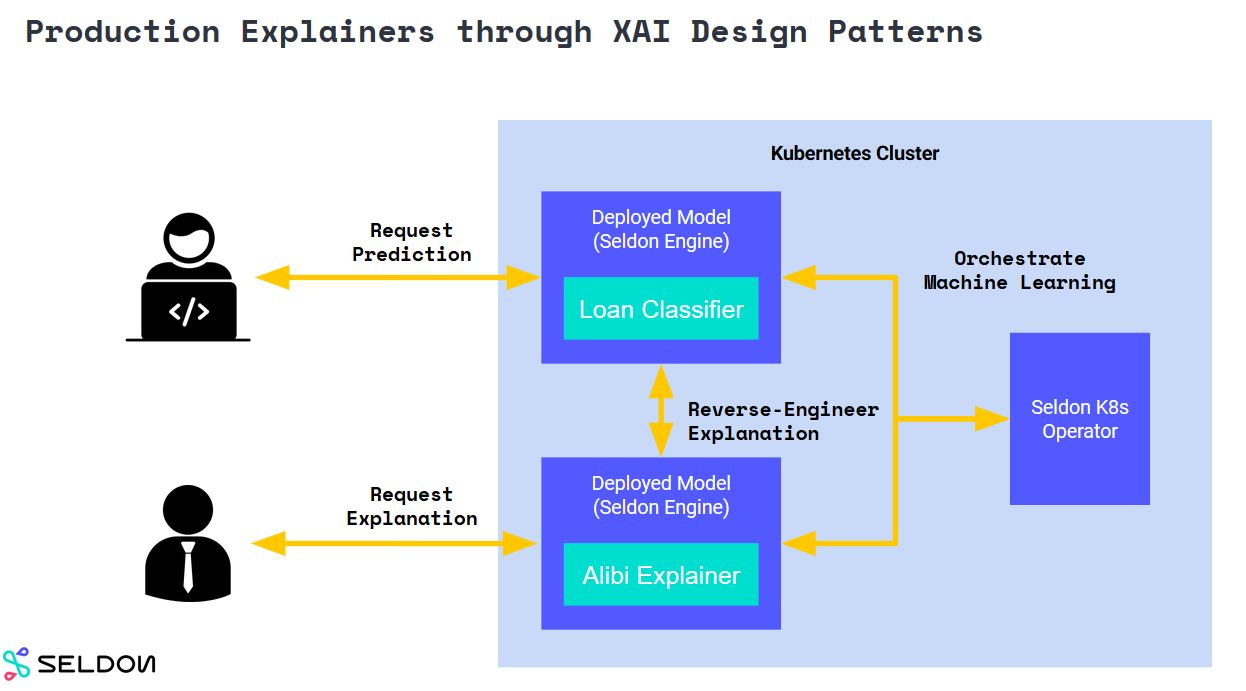
Visualise metrics and explanations

Revisiting our workflow